If accurate color is a must in your world, then you know the importance of color measurement instrumentation.
Spectrophotometers are used in many industries to identify, formulate, measure and communicate color. They can compare samples and standards to identify even the smallest differences. From concept through formulation and production, spectrophotometers are an invaluable part of any color-managed workflow.
But have you ever stopped to think how these devices were developed? Today we’ll take a trip back in time to meet the brains behind the research and the experiments that paved the way for color measurement devices.

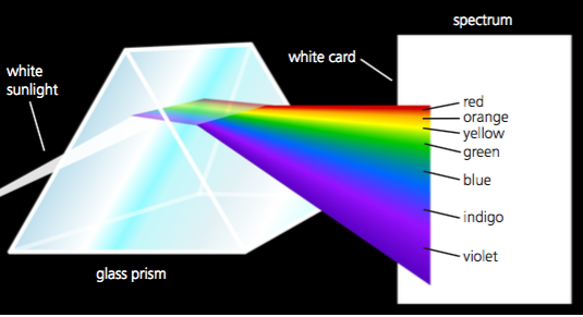
Isaac Newton used a prism to refract white light into the colors of the visible spectrum. Used with permission from Wikipedia
Isaac Newton: The many colors of light
Although mankind had a vague understanding that light was at least partially responsible for color, it was Isaac Newton (1642-1727) who used glass prisms to demonstrate that a beam of white light could be separated into the visible spectrum. His experiments with refracting and bending a light’s path to break it into individual components gave us a meaningful way to describe the range of colors we can see with ROY G. BIV – red, orange, yellow, green, blue, indigo and violet. With this knowledge, Newton developed the Newton Color Circle, which began interesting research into complementary colors and additive color mixing.
Thomas Young: Our color-mixing eyes
In the very early 1800’s, Thomas Young shared his belief that the human eye contains three different types of color receptors that are used to mix red, green and blue to create the wide range of colors we can see. He was right.
James Clerk Maxwell: Electromagnetic energy
 James Clerk Maxwell continued that thought in the 1860’s by demonstrating that combinations of red, green, and blue could be used to create almost any other desired color. He realized it wasn’t possible to combine these three primary colors into the entire gamut of hues, but soon learned that with some subtraction, the entire gamut could be achieved. Today, this phenomenon is known as the human tristimulus response.
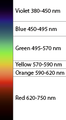
Although he was not the first to propose a “wave” theory of light, Maxwell was able to demonstrate that light is a form of electromagnetic energy that can be quantified in wavelengths between 380 (violet) and 750 (red) nanometers (nm). Today we use this scale to assign specific numbers to points of the visible spectrum… much more precise than Newton’s Roy G. Biv!
What about those wavelengths below 380 and above 750? Maxwell theorized that they exist, but our eyes can’t see them. Today we know the wavelengths higher than 750 as infrared, and below 380 as ultraviolet.
Maxwell also recognized that a color’s hue and saturation – known as chromaticity – are independent from brightness… providing an early peek at what would develop into the CIE chromaticity diagram.
Guild & Wright: Color spaces
In the late 1920’s, W. David Wright and John Guild continued the quest with experiments to evaluate how much red, green, or blue light energy was necessary to see any color across the visible spectrum. Their work taught us that there is a link between color wavelengths in the visible spectrum and the colors the human eye can perceive.
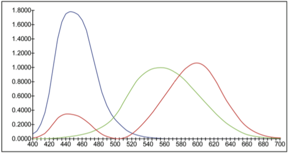
This graph shows the amount of red, green or blue light energy needed to match any color across the visible spectrum.
The Commission International de l’Eclairage (CIE) published Guild and Wright’s research as the 1931 RGB Color Space, which led to the CIE 1931 XYZ Color Space. Although these mathematical equations helped us quantify the human visual response to color and are the basis for color measurement devices, it didn’t take long for scientists to realize that the two-dimensional model comprised of so much green wasn’t perfect.

Published around the same time as the CIE 1931 Color Space, the CIE chromaticity diagram was a 2-dimensional attempt to document colors on a graphic scale.
David MacAdam: Tolerancing
Color was a very interesting topic to David MacAdam, who worked for Kodak in the 1940’s. He wanted to know how much he could change the color of Kodak Yellow before observers would notice a difference. From master (target) samples, he changed the hue, chroma (or saturation) and lightness until his observers noted a difference. He then plotted the results on the CIE chromaticity diagram. He repeated this experiment for a large assortment of colors, creating the first-ever tolerancing diagram.
In each case, the distribution of matching points formed a three-dimensional ellipse, or ellipsoid. Interestingly, the ellipsoids were different sizes depending on the position of the color in color space. MacAdam showed that the chromaticity diagram is not uniform, and in order for it to be used as a color tolerancing tool, different tolerance values must be specified for each color. The results also proved that our eyes do not weight hue, lightness, and chroma equally… the human eye is about twice as sensitive to hue shifts as it is to shifts in chroma or lightness.
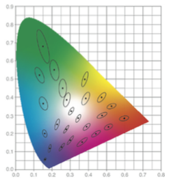
These perceptibility limits around each color target show the amount of difference that is allowed before the human eye will notice.
From MacAdam’s work, we know that color difference tolerancing requires larger ellipses for some colors, and smaller ellipses for others, and that a 2D graph just won’t work.
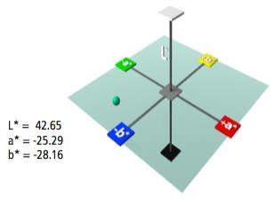
Richard Hunter: L*a*b*
Using MacAdam’s work, Richard Hunter created a new tristimulus color model in the 1940’s. This color space, which he called L*a*b*, uses three axes to represent near uniform spacing of perceived color difference. Vertical L represents lightness/darkness with white at 100 and black at 0 and shows differences between dark colors and lighter pastels. Horizontal and perpendicular, a and b, represent the major color axes, with red at positive a with green at negative a; and yellow at positive a with blue at negative b.
With this color model, Hunter developed a way to plot exact colors in color space and characterize total color difference using Delta E. If you’d like to learn more about CIE L*a*b* and tolerancing, check out our recent post.
Thirty-one years later, the CIE published an updated model – CIE L*a*b* – with only a few small changes to Hunter’s original math. Today it is the recommended method for reporting colorimetric values, and the math that is used by many of our color measurement instruments.
Tolerancing in CIE L*a*b*.
Putting it all to use
This path of realization, from light, to color mixing, to the visible spectrum, to color models and tolerancing, is the foundation for today’s color measurement instruments. Learn more by reading our Modern Instrumentation post to learn how all of this research is used to provide a scientific way for quantifying, judging, and communicating color.